Relative Motion Analysis Using Vectors
This section presents relative motion using vector notation.
Relative motion analysis is one method used to analyze bodies undergoing general planar motion. General planar motion is motion where bodies can both translate and rotate at the same time. Besides relative motion analysis, the alternative is absolute motion analysis. Either method can be used for any general planar motion problem, however one method may be significantly easier to apply in certain situations.
Absolute motion analysis will require calculus and is generally faster for simple problems and problems where only the velocities (and not accelerations) are required. Relative motion analysis will not require calculus, but does necessitate using multiple coordinate systems and is generally easier to use for more complex problems and problems where velocities and accelerations are being analyzed.
Utilizing Relative Motion Analysis
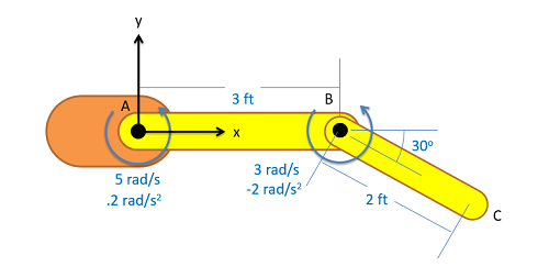
To start our discussion on relative motion analysis, we are going to imagine a simple robotic arm such as the one below. In this arm, we have a two arm sections of fixed length with motors causing rotations at joint A and joint B.
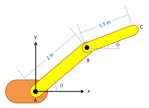
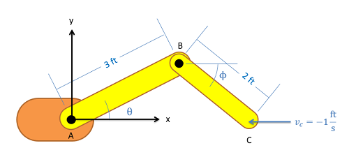
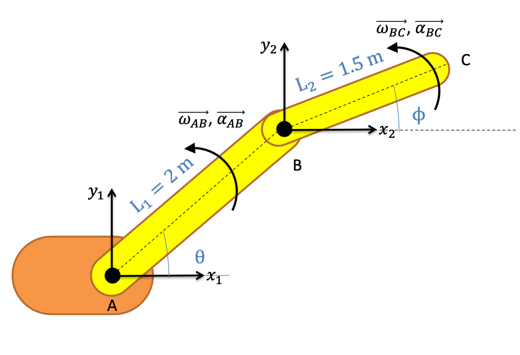
The first step in relative motion analysis is to break the motion down into simple steps and assign a translating coordinate system (with x and y directions) attached to points of interest along the rigid bodies. Note that this coordinate system will translate with the point of interest, but will not rotate with the object. (We will use rotating coordinate systems later for more complex problems in the rotating frames method). We will typically start at a point with known motion (or a fixed point) and move step by step from there. In the case of our robotic arm, we know Joint A will not be moving so we start there. We will determine the velocity at point B (with respect to point A), and then point C (with respect to point B).
Below is a picture of the robotic arm with the coordinate systems drawn in.
For relative motion analysis, we can identify the velocity or acceleration of the end point of the arm (C) with respect to the ground (A) by finding the velocity acceleration of B with respect to A and adding the velocity or acceleration of C with respect to B, just as we did with particles. Note that velocities that are relative to the fixed coordinate system are often designated with one subscript, and considered absolute velocities and accelerations.
| Velocity: | \[\vec{v}_{C/A}=\vec{v}_{B/A}+\vec{v}_{C/B}\] |
|---|---|
| or | \[\vec{v}_{C}=\vec{v}_{B}+\vec{v}_{C/B}\] |
| Acceleration: | \[\vec{a}_{C/A}=\vec{a}_{B/A}+\vec{a}_{C/B}\] |
| or | \[\vec{a}_{C}=\vec{a}_{B}+\vec{a}_{C/B}\] |
The relative motion analysis equations above are for a two-part motion (there are two sections to the arm in our example) but we can easily expand the above equation into three, four, or even more pieces for more complex mechanisms by adding more steps to the left side of our equation.
To use the above equations, we will need to plug in the information we know. Plugging in velocities or accelerations that are given as part of the problem for any particular points is a good place to start. If the velocity of points B or C were given for example, we would plug that in for vB or vC respectively. Do remember that point A is our fixed ground point so vC is the velocity of point C relative to the ground, while vC/B is the velocity of point C with respect to point B. If any point is fixed (other than our original ground point, which will always be fixed) we can also plug in zeros for both velocity and acceleration of that point. Do remember the above equation is a vector equation, so these velocities have both a magnitude and a direction.
In some cases, we want to analyze multiple points on the same or several rigid bodies. Another notation used for this is:
| Position: | \[\vec{r_B} = \vec{r_A} + \vec{r_{B/A}}\] |
|---|---|
| Velocity: | \[\vec{v_B} = \vec{v_A} + \vec{v_{B/A}} = \vec{v_A} + \vec{\omega} \times \vec{r_{B/A}}\] |
| Acceleration: | \[\vec{a_B} = \vec{a_A} + \vec{a_{B/A}} = \vec{a_A} + \vec{\alpha} \times \vec{r_{B/A}} + \vec{\omega} \times (\vec{\omega} \times \vec{r_{B/A}}) \] |
In this notation, A and B are two points on the same rigid body. When we use only one subscript, that indicates the position/velocity/acceleration of that point with respect to the fixed coordinate system. Because the body is rigid, the two points will not change the distance between them, but the position vector between them can change orientation (which is where the relative velocity between the two points comes from). Omega is the angular velocity of that rigid body (analogous to theta dot) and alpha is the angular acceleration of that rigid body (analogous to theta double dot).
For planar motion, where the angular velocity vector (out of plane) is always perpendicular to the position vector (in the plane), the acceleration can be simplified to:
| Acceleration: | \[\vec{a_B} = \vec{a_A} + \vec{\alpha} \times \vec{r_{B/A}} - \omega^2 \vec{r_{B/A}} \] |
|---|
All vectors will be defined with respect to the x and y coordinates in the coordinate system shown, rather than the radial and theta directions as above.
If we want to find the velocity and acceleration of the end point, C, knowing the angular velocities and accelerations, we will find the following relationships:
| Velocity at point B: | \[\vec{v_B} = \vec{v_A} + \vec{\omega_{AB}} \times \vec{r_{B/A}}\] |
|---|---|
| Velocity at point C: | \[\vec{v_C} = \vec{v_B} + \vec{\omega_{BC}} \times \vec{r_{C/B}}\] \[= \vec{v_A} + \vec{\omega_{AB}} \times \vec{r_{B/A}} + \vec{\omega_{BC}} \times \vec{r_{C/B}}\] |
| Acceleration at point B: | \[\vec{a_B} = \vec{a_A} + \vec{\alpha_{AB}} \times \vec{r_{B/A}} - \omega_{AB}^2 \vec{r_{B/A}} \] |
| Acceleration at point C: | \[\vec{a_C} = \vec{a_B} + \vec{\alpha_{BC}} \times \vec{r_{C/B}} - \omega_{BC}^2 \vec{r_{C/B}} \] \[ = \vec{a_A} + \vec{\alpha_{AB}} \times \vec{r_{B/A}} - \omega_{AB}^2 \vec{r_{B/A}} + \vec{\alpha_{BC}} \times \vec{r_{C/B}} - \omega_{BC}^2 \vec{r_{C/B}} \] |
Once we have everything in our vector equation, we will break the vector equation into x and y components in order to solve for any unknowns. Simply find the angles or each of the r and theta directions using your diagram and use sines and cosines to break the individual vectors down into x and y components. Once you have everything in component form, you should be able to solve for any unknowns in your equations. As a note, it is often necessary to start with the velocity equations and solve for some unknowns there before moving on to the acceleration equations.