Two Dimensional Kinematics in Rectangular Coordinate Systems
Two Dimensional Motion (also called Planar Motion) is any motion in which the objects being analyzed stay in a single plane. When analyzing such motion, we must first decide the type of coordinate system we wish to use. The most common options in engineering are rectangular coordinate systems, normal-tangential coordinate systems, and polar coordinate systems. Any planar motion can potentially be described with any of the three systems, though each choice has potential advantages and disadvantages.
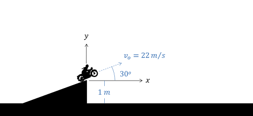
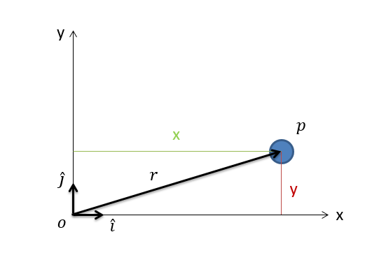
The rectangular coordinate system (also sometimes called the Cartesian coordinate system) is the most intuitive approach to describing motion. In rectangular coordinate systems we have an x and a y axis. These axes remain fixed to some origin point in the environment and they do not change over time. Instead, the bodies we are analyzing usually move relative to these fixed axes. An example of a body with a rectangular coordinate systems is shown in the figure below.
Rectangular coordinates work best for systems where all forces maintain a constant direction. The most common example of this is projectile motion, where gravity (the only force in these systems) maintains a constant downward direction. An example of a system where the forces change direction over time would be something like a car going around a curve in the road. In this case the friction force at the tires is going to be rotating with the car. The car problem will therefore be better suited to the use of normal-tangential or polar coordinate systems.
When describing the position of a point in rectangular coordinate systems, we are going to start by describing both x and y coordinates in a vector form. For this, the values x and y represent distances and the unit vectors i and j are used to indicate which distance corresponds with which direction. This may seem redundant, but remember when solving actual problems, x and y will just be numbers.
| Position: | \[r_{p/o}(t)=x(t)\hat{i}+y(t)\hat{j}\] |
|---|
Just as with one dimensional problems, if we take the derivative of the position equation, we will find the velocity equation. If we take the derivative of the velocity equation we will wind up with the acceleration equation. Also like one dimensional problems, we can use integration to move in the other direction, moving from an acceleration equations to a velocity equation to a position equation.
The unit vectors add a new element in two dimensions, but since the unit vectors don't change over time (aka. they are constants), we treat them like we would any other constant for derivatives and integrals. The resulting velocity and acceleration equations are as follows.
| Velocity: | \[v(t)=\dot{x}(t)\hat{i}+\dot{y}(t)\hat{j}\] |
|---|---|
| Acceleration: | \[a(t)=\ddot{x}(t)\hat{i}+\ddot{y}(t)\hat{j}\] |
The above equations are vector equations with velocities and accelerations broken down into x and y components. Since the x and y directions are perpendicular, they are also independent (movement in the x direction doesn't impact movement in the y direction and vice versa). This essentially means we can split our vector equation into a set of two scalar equations. To do this we just put everything in front of the i unit vectors in the x equations and everything in front of the j unit vectors in the y equations.
| Position: | \[x(t)=...\] | \[y(t)=...\] |
|---|---|---|
| Velocity: | \[\dot{x}(t)=...\] | \[\dot{y}(t)=...\] |
| Acceleration: | \[\ddot{x}(t)=...\] | \[\ddot{y}(t)=...\] |
Once we have the everything split into x and y directions we can just use the same processes we used for one dimensional motion to move from x, to x dot, to x double dot and from y, to y dot, to y double dot. The variable linking the two equations is time t, or time in both the x and y equations.